Audio Workshop 14

Data Analysis – Fourier Transform

Fourier transform gives you detailed analysis of the audio spectrum. it turns data in time to data in frequency, which is really useful for building an art installation or costume that reacts uniquely to sounds in different frequency ranges.

The acronym FFT means Fast Fourier Transform, which refers to a mathematical optimization. FFTs have two types of output. Complex output gives you 2 numbers per frequency, and is generally needed if you will turn the frequency data back into an audio signal. The Teensy Audio Library provides the simpler Real output, where you get a single number per frequency. The numbers tell you the amount of signal found at each frequency, without any information about its phase shift.

Design the Audio System

To begin exploring Fourier transform, draw the simple system below. Even with FFT optimization, a 1024 point analysis (which provides detailed results) will require significant computational power, so only a single fft1024 object is used. The stereo WAV file is mixed to mono for the sake of the analysis.

Turn the Design into Code and Use it in a Program

Unlike most of our previous examples, we are going to use the example program “Part_3_02_Fourier_Transform” from the examples in the IDE . Go to File > Examples > Audio > Tutorial > Part_3_02_Fourier_Transform to open.

You’ll notice that the program has multiple tabs in addition to the main program which contain some of the sound data. That is why we are using the example from the IDE rather than rolling our own.

Once the program is open, we will need to manually change the buttons from pins 0-2 to 3-5 as we did in the other examples as shown here because we will make use of them in this tutorial.

// Bounce objects to read pushbuttons 
Bounce button0 = Bounce(3, 15);
Bounce button1 = Bounce(4, 15);  // 15 ms debounce time
Bounce button2 = Bounce(5, 15);

void setup() {
  pinMode(3, INPUT_PULLUP);
  pinMode(4, INPUT_PULLUP);
  pinMode(5, INPUT_PULLUP);

We also need to initialize the LCD to prevent any conflict with the SD card on the Audio Adapter by adding the code below as you have seen in many other examples.

#include <ILI9341_t3.h>
#include <font_Arial.h>
#include <XPT2046_Touchscreen.h>

// LCD control pins defined by baseboard
#define TFT_CS 40
#define TFT_DC  9

// Use main SPI bus MOSI=11, MISO=12, SCK=13 with different control pins
ILI9341_t3 tft = ILI9341_t3(TFT_CS, TFT_DC);

// Touch screen control pins defined by baseboard
// TIRQ interrupt if used is on pin 2
#define TS_CS  41
//#define TIRQ_PIN  2 
XPT2046_Touchscreen ts(TS_CS);  // Param 2 = NULL - No interrupts

void setup() {
  Serial.begin(9600);

  // Setup LCD screen
  tft.begin();
  tft.setRotation(3);
  ts.begin();
  ts.setRotation(1);
  tft.fillScreen(ILI9341_BLUE);

Alternatively you can use the SD card on the Teensy 4.1 if you don’t want to mess with initializing the LCD.

Now Export and copy & paste the code into the program in the usual place and verify and upload the completed program to the Teensy.

Looking at the Fourier Transform Output Data

When the code runs, this should appear in the Serial Monitor window with lots of data going by very fast.

The FFT analysis produces a tremendous amount of data. This rapidly scrolling window shows only the first 30 of the 512 frequency “bins” arranged in 30 columns. However, these 30 are much more important than the remaining 482. Later we’ll look at why that is. For now, let’s concentrate on understanding these numbers.

Each frequency bin represents the amount of signal found at a particular frequency. The bins are spaced 43Hz apart because the audio has a 44.1kHz sampling rate / 1024 FFT points = 43Hz.

• Bin 0 = DC or zero Hz component
• Bin 1 = 43Hz
• Bin 2 = 86Hz
• Bin 3 = 129Hz
• Bin 4 = 172Hz
• Bin 5 = 215Hz
• Bin 6 = 258Hz
• etc …

The numbers are typically small. You may recall from Workshop 6 – Mixers that signals range from -1.0 to 1.0. The FFT considers only the total amount, so you get only positive numbers. If a signal total is 1.0, meaning it is actually oscillating between -1.0 to 1.0, the FFT will report it as 1.0, likely spread across many bins if it’s composed of many frequencies.

For example, consider a signal with a total amplitude of 0.6 composed of a mixture of 25% 120Hz and 75% 1kHz. Bins clustered around 3 (129Hz) and around 23 (989Hz) will indicate the amount of each part. Bin 3 and nearby bins will sum to 0.15 (25% of 0.6) and bin 23 and nearby bins will sum to 0.45 (75% of 0.6). The sum of all bins always equals the total amount of the signal. There are finer details to consider, but first let’s do some listening tests to see the data corresponding to real sounds.

Guitar Listening Test

If you press the 3 buttons, you’ll hear that each activates one of the 3 signal sources you drew in the design tool. The left (BTN0) plays the 4 wave files, changing with each button press, middle (BTN1) plays a guitar sample and right (BTN2) plays a sine wave tone. When you listen to the guitar sample from the middle (BTN1) button, you should see something like this:

After the sound stops, it’s easy to scroll up and see the notes. In this screenshot, you can see a moment where the string is plucked, which results in a few lines with rapidly changing numbers in many frequency bins. Then the guitar string vibrates with at least 4 frequency ranges (visible in this data). Soon the higher frequency components fade as the guitar string vibration settles towards the wavelength matching the string length between the player’s finger and the bottom of the instrument.

Experiment with Thresholds for Data Visualization

Visually detecting patterns in FFT data of composed music is much harder than a single instrument. The many separate sounds often overlap in frequency bins. Human hearing and the brain’s ability to discern complex combinations of sounds is pretty amazing.

To improve things a bit, find the printNumber() function near the end of the example. This print function has a threshold of 0.004 which means it will only print numbers above that value.

void printNumber(float n) {
  
  if (n >= 0.004) {
    Serial.print(n, 3);
    Serial.print(" ");
  } else {
    Serial.print("   -  "); // don't print "0.00"
  }

Edit the threshold and increase it from 0.004 to 0.024. By increasing the threshold, it will print less detail, allowing you to more easily see the numbers for only the stronger sounds.

The first song that automatically plays is “Where You Are Now” featuring WolfSky singing. She has a strong voice, which usually shows up as distinct columns of numbers scrolling by.

Unlike the acoustic guitar piece played from the middle button, the guitars and other instruments in this music have many complex effects applied. Those effects which produce rich and complex sounds tend to scatter the instrument’s numbers across many frequency bins. Because the bins add up to the signal’s total, the numbers in most bins are lower, mostly below this higher 0.024 threshold.

You can try adjusting the threshold to see if other types of sounds become noticeable in the scrolling data.

The printNumber() function also has alternate ASCII art code you can try at the bottom of the program and perhaps even extend or redesign with other patterns to better see the relative signal strength in each bin.

Scrolling numbers probably won’t impress many people (unless they are fans of the Matrix), but perhaps instead of printing to the serial monitor, you could turn LEDs on/off, animate RGB LEDs to different colors or control solenoids and motors to visualize the music.

Understanding FFT Mathematical Limitations

The right (BTN2) button plays pure sine waves. Each time you press it, you’ll hear a higher pitch, until it cycles through all 12 musical notes. The notes play for as long as you hold the button. The exact 12 frequencies it plays are determined by this array.

int noteNumber = 0;
const float noteFrequency[12] = {
  220.00,  // A3
  233.08,  // A#3
  246.94,  // B3
  261.63,  // C4
  277.18,  // C#4
  293.66,  // D4
  311.13,  // D#4
  329.63,  // E4
  349.23,  // F4
  369.99,  // F#4
  392.00,  // G4
  415.30   // G#4
};

If you previously edited the printNumber() threshold, restore it back to 0.004.

Press and hold the right button. When Teensy plays 220Hz (musical note A3), you will see this.

This example shows a limitation of the Fourier transform. For signal frequencies which don’t align perfectly on the FFT bin frequencies, you can never have ideal performance.

Windowing Reduces Leakage

Windowing in FFT lingo refers to algorithms that limit the data so that it stays within a range (or window) of bins.

By default, the fft1024 object uses a Hanning window, which causes frequencies not exactly on a FFT bin to cluster in the close-by bins, but also smears the data across several nearby bins. Ideally, you’d like your 220Hz frequency to appear mostly in the 215Hz bin, with some perhaps also in the 259Hz bin. The Hanning window gets you close, with 0.496 in the 215Hz bin and 0.290 in the 258Hz bin. But 0.211 ends up in the 172 Hz bin, and small amounts also go to the 129 and 301Hz gins, which isn’t so desirable. They still add up to 1.0, the original signal size, but they’re smeared across 5 bins instead of the desired 2.

You can disable the Hanning window by editing this code. Just uncomment the line which sets the window to NULL

  // Uncomment one these to try other window functions
   fft1024_1.windowFunction(NULL);
  // fft1024_1.windowFunction(AudioWindowBartlett1024);
  // fft1024_1.windowFunction(AudioWindowFlattop1024);
  delay(1000);

Now when you press the button for 220Hz sine wave tone, you should see this with the window disabled.

At first glance, this looks pretty horrible. But if you read the actual numbers, you’ll see the 215Hz bin has numbers between 0.971 and 0.992. The 258Hz bin is between 0.108 and 0.126. So almost all of our 220Hz sign wave did go into the 2 desired bins. However, some of it got scattered across almost all the other bins. The problem is called Spectral Leakage. The windows are meant to prevent spectral leakage, by containing all the results to only nearby frequency bins.

To understand how a pure 220Hz sine wave becomes data in all those other frequency bins, consider this plot of 4096 points of a 220Hz sine wave, sampled at 44.1kHz.

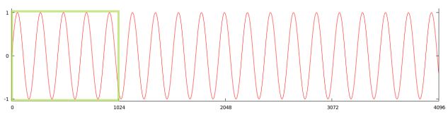
The green box is 1024 points where the FFT analyzes the spectrum. The FFT reports the spectrum based on the assumption the waveform is periodic, that it repeats indefinitely.

Here is the same 220Hz waveform with the first 1024 point section repeated 4 times. Without a window, the FFT is returning the spectrum of this waveform, which differs from the intended 220Hz pure sign wave shown above.

The window function is just another waveform which the signal is multiplied by, before the FFT. the Hanning window is basically just an offset sine wave, which multiplies the original waveform by zero at the beginning and end of the window and by 1 in the middle.

Window functions destroy about half the original data, where they multiply by zero or very small numbers. For this reason, the Teensy Audio Library uses 50% overlap in its fft1024 object. Twice as many 1024 point FFTs are computed, where the second set uses the window function offset by 512 points.

With the pure 220Hz tone, the graph below shows the actual windows inputs to each 1024 point Fourier transform.

A new 1024 point FFT is completed every 512 samples, because they are performed at twice the rate on 50% overlapping data after windows are applied.

Because of the 50% overlap, fft1024_1.available() will return true 86 times per second. Each new update of fft1024 data represents the prior 1024 samples (approximately 23.2ms) with a window applied, so it was most sensitive to the sound in the center of those 23.2ms.

Many different window shapes are available in the library, which trade off spectral leakage versus smearing of the frequency bins. A couple of them can be uncommented in the code to try them out.

  // Uncomment one these to try other window functions
  // fft1024_1.windowFunction(NULL);
  // fft1024_1.windowFunction(AudioWindowBartlett1024);
   fft1024_1.windowFunction(AudioWindowFlattop1024);
  delay(1000);

There is no magic solution if your signals have frequencies no perfectly aligned onto the FFT bins. But despite these limitations, the FFT works great for sound reactive projects.

Next up, we’ll take a look at data visualization using our LCD display.